Feature visualisation

A great tool for interpreting neural networks is feature visualistion, which allows us to inspect what each neuron is activating for.

This post explores the tricks in Chris Olah’s Feature Visualisation work. We focus on visualising the classes, rather than hidden neurons.

We’ll use an image classifier trained on CIFAR10. Images are 32x32, and there are 10 possible classes. We train on 50,000 images, and achieve ~70% accuracy on the test set. One of the most suprising take aways from this work is that a relatively low-quality dataset and far from SOTA model can still have interpretable feature visualisations.

Optimising images, not weights

We want to visualise what a neuron is activated by. We can do this by maximising the neuron’s activation by optimizing the input image (in the same way we usually minimise the cost function by optimising the model’s weights).

model_sliced = torch.nn.Sequential(*model[:layer_idx + 1])

# Start with a small amount of random noise.
input = torch.normal(mean=0, std=0.1, size=(1, 3, 32, 32))
input = torch.nn.Parameter(input, requires_grad=True)

optimizer = torch.optim.Adam([input], lr=0.05)

for step in range(1500):
  optimizer.zero_grad()
  layer_activations = model_sliced(input_mod)
  neuron_activations = layer_activations[:, neuron_idx]
  cost = (-neuron_activations).sum()
  cost.backward()
  optimizer.step()

Diverse images

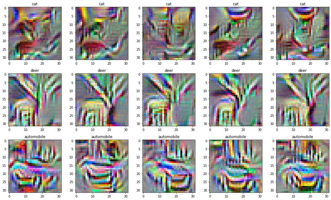
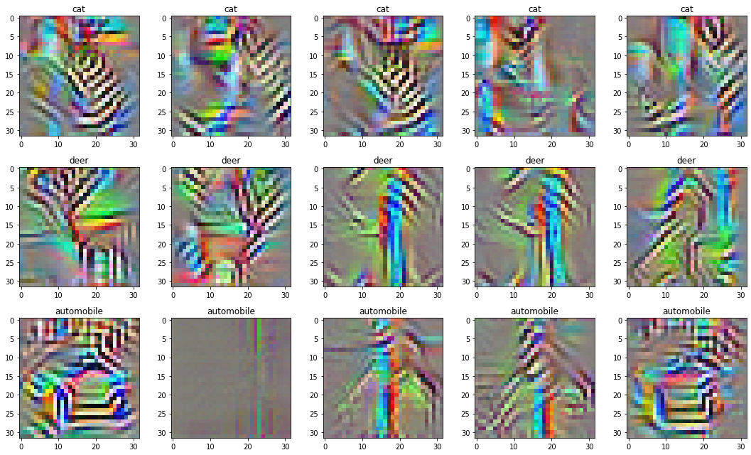
We can create a range of visualisations by repeating the process above with different random initial noise. To increase the diversity of the generated images, we can add a term to the cost function.

We calculate this by:

• For each image in the dataset…
  • Take a hidden layer’s activations. We find that the first layer works well here.
  • Calculate the covariance matrix across features:
    • Given activations \(A_{x \times y \times c}\).
    • Flatten to \(A_{n \times c}\) where \(n = x \times y\).
    • Calculate the covariance matrix \(C_{c \times c}\).
    • Flatten the covariance matrix to \(C_n\) where \(n = c \times c\).
• Sum the cosine similarities between each image:
  • \(\sum_{i} \sum_{j \neq i} \frac{C_n^i C_n^{j}}{||C_n^i||||C_n^j||}\)
• Add this value to the cost function.

This is implemented as:

x = torch.flatten(hidden_layer_activations, 1, 2)
x = x.permute(0, 2, 1) @ x
x = torch.nn.functional.normalize(x, p=2, dim=(1, 2))
diversity_cost = sum([
    (x[i] * x[j]).sum()
    for i in range(NUM_IMAGES_PER_NEURON)
    for j in range(NUM_IMAGES_PER_NEURON)
    if i != j
]) / NUM_IMAGES_PER_NEURON

By doing this, we end up with the following collection of images:

Not great.

Tricks

Chris Olah’s work employs a few tricks: augmentation, Fourier parameterisation, and decorrelating colors.

Trick 1: Augmenting

One problem is that the image we’ve created has “overfit” to the neuron. We can apply some random augmentations to the input image to fix this.

• Padding the image by 3, just to help with edge artifacts.
• Randomly translating the image by \([-8, 8]\) along each axis.
• Randomly rotating the image by \([-5, 5]\) degrees.
• Randomly scaling the image by \([0.95, 1.05]\).

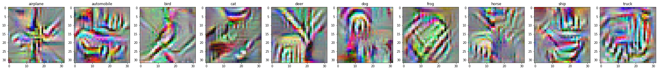
This helps a lot! I find this is the most important trick, and gets you 80% of the way to a good looking solution.

Note that the augmentations happen within the forward and backward pass: the gradients flow through the transformation to the visualisation.

# ...
input = torch.normal(
    # Start with a small amount of random noise.
    mean=0, std=0.1,
    # Add 3 to the image size to avoid edge artifacts when randomly
    # transforming the image.
    size=(1, 3, 32 + 3 * 2, 32 + 3 * 2))
# ...
input = torchvision.transforms.functional.affine(
    input,
    translate=[random.randint(-3, 3), random.randint(-3, 3)],
    angle=random.uniform(-5, 5) / 360 * (2 * math.pi),
    shear=[0, 0],
    scale=random.uniform(0.95, 1.05),
)
input = torch.nn.functional.pad(input, (-3, -3, -3, -3))

Trick 2: Fourier parameterisation

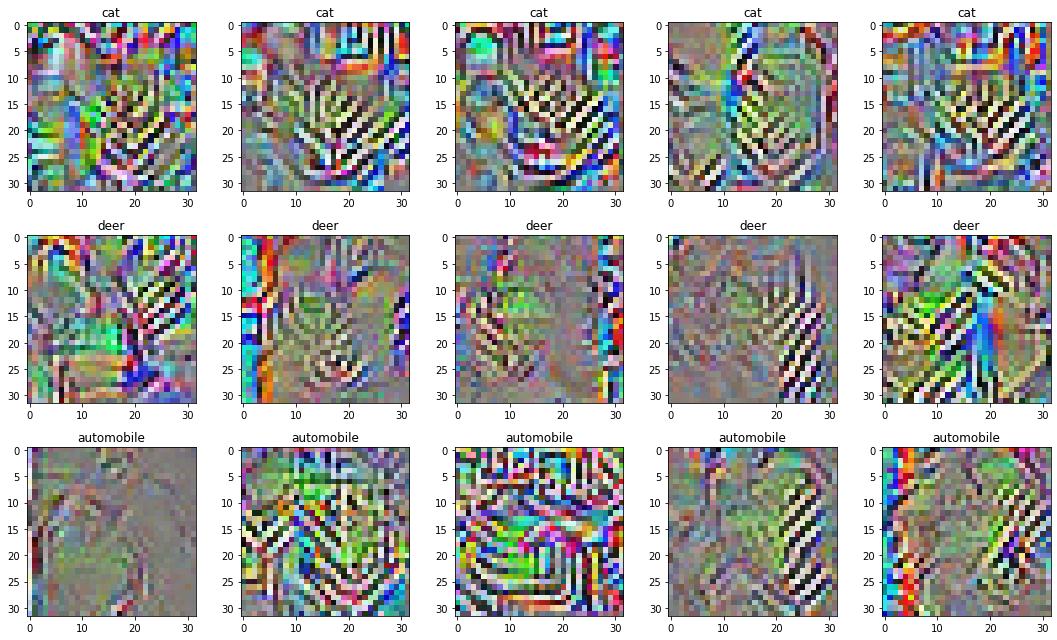
The above visualisations overuse high frequency patterns, especially in backgrounds. We can reduce this by parameterising the image as its Fourier transform, and scaling this parameterisation.

We still have a \(I_{x \times y \times c}\) matrix to represent the image. But instead of \((x, y)\) representing the location of a pixel, it represents a frequency.

We reduce high frequencies by (1) finding out the frequency represented by each \((x, y)\) value, and (2) scaling each value by the inverse of the frequency.

parameters = np.random.normal(size=(2, num_images, 3, size, size), scale=0.01)
parameters = torch.tensor(parameters).cuda()
parameters = torch.complex(parameters[0], parameters[1])
parameters = torch.nn.Parameter(parameters, requires_grad=True)
...
# Find what frequencies each [x, y] value corresponds to.
freqs_y = torch.fft.fftfreq(size)[:, None]
freqs_x = torch.fft.fftfreq(size)
freqs = torch.sqrt(freqs_x * freqs_x + freqs_y * freqs_y).cuda()
# Scale the spectrum. First normalize energy, then scale by the square-root
# of the number of pixels to get a unitary transformation.
# This allows to use similar learning rates to pixel-wise optimisation.
scale = 1.0 / torch.maximum(freqs, torch.tensor(1.0 / size))
scale *= np.sqrt(size * size)
parameters = torch.tensor(scale) * parameters
# Translate to spacial representation.
image = torch.fft.ifft(parameters).real

This goes a long way in reducing the high frequencies. However, this doesn’t make high frequencies impossible to get to. You can think of this as stretching the loss landscape to make it take a longer time to get to high frequencies.

Trick 3: Decorrelating the colors

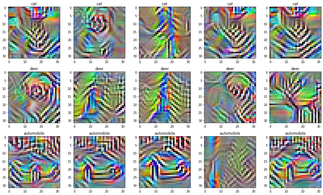
Finally, the colors are really vivid. To fix this, we decorrelate the colors. This is done to the dataset before training the model.

We do this by applying a whitening transformation. Our goal is for the model to see colors that have the identity \(I_{3 \times 3}\) covariance matrix.

• Given a dataset \(D_{s \times x \times y \times c}\) where \(s\) is the number of samples.
• Flatten to \(D_{n \times c}\) where \(n = s * x * y\).
• Calculate the covariance matrix \(C_{c \times c}\).
• Calculate the Cholesky decomposition \(L^{T}L = C_{c \times c}\).
  • \(L\) is an upper triangular square root of \(C\).
• Transform the original dataset by the inverse of the Cholesky decomposition:
  • \(D'_{s \times x \times y \times c} = D'_{s \times x \times y \times c} inv(L^T)\).
• \(D'\) should now have the identity covariance matrix.

def _get_color_cov(images: np.ndarray) -> np.ndarray:
  colors = images
  colors = np.transpose(images, (1, 0, 2, 3))
  colors = colors.reshape((3, -1))
  color_cov = np.cov(colors)
  return color_cov

def _get_decorrelating_transform(cov: np.ndarray) -> np.ndarray:
  cov_inv = np.linalg.inv(cov)
  cholesky = scipy.linalg.cholesky(cov_inv)
  return cholesky.T

def _transform_colors(images: np.ndarray, transform: np.ndarray) -> np.ndarray:
  # Wrap in permutations so that the matmul'd dimension is last.
  images = np.transpose(images, (0, 2, 3, 1))
  images = images.dot(transform)
  images = np.transpose(images, (0, 3, 1, 2))
  return images

color_cov = _get_color_cov(train_input_raw)
decorrelating_transform = _get_decorrelating_transform(color_cov)
decorrelating_transform_inv = np.linalg.inv(decorrelating_transform)

train_input_decorrelated = _transform_colors(
    train_input_raw, decorrelating_transform)
test_input_decorrelated = _transform_colors(
    test_input_raw, decorrelating_transform)

Much better: